Bayesian Flow Networks (BFNs) link iterative denoising diffusion and recursive estimation of distribution parameters.
At \(t = 0\) we initialize independent and identically distributed parameters from a chosen family. A neural network mixes independent distribution parameters. Mixed parameters are used to perform updates using the Bayes rule. Finally, at \(t = 1\) the parameters represent a particular example in the larger data distribution.
In autoregression, you train on trajectories that realize one variable at a time with teacher forcing. In BFNs a single forward pass of the network predicts a small update to parameters of the joint distribution of all variables, and realization is done using plain Bayesian posterior update rules. The amount of updates you choose to make is not dependent on how many variables your sequence has.
In this post, I’ll sketch a tiny BFN that uses Siren-guided Gaussian update rules to model a mixture of Gaussians.
Code
import mathimport matplotlib.pyplot as pltimport torchimport torch.nn as nnplt.rcParams['axes.spines.left'] =Falseplt.rcParams['axes.spines.right'] =Falseplt.rcParams['axes.spines.top'] =Falseplt.rcParams['axes.spines.bottom'] =False
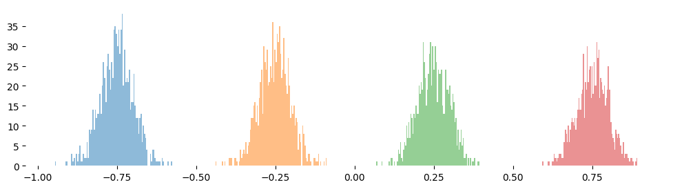
Let’s define the large data distribution: a mixture of one-dimensional Gaussians.
torch.manual_seed(3407)dataset = []plt.figure(figsize=(12, 3))for mean in [-0.75, -0.25, 0.25, 0.75]: mu = mean + torch.randn(1000) *0.05 plt.hist(mu, bins=100, alpha=0.5) dataset.append(mu)dataset = torch.cat(dataset, dim=0).unsqueeze(-1)
Siren
Let’s define the approximator \(f_\theta\). Given input distribution parameters \(\mu\) and a timestamp \(t\), a neural network will approximate output distribution parameters.
I will use a Siren, an MLP that uses a sin activation function with a large scale on the activations, artificially amplifying their frequency before applying the sine. The scale is commonly called “bandwidth” in the GP kernels literature.
This way the MLP will be biased towards wiggly functions and will be able to represent time without relying on hardcoded positional encodings – let the Siren find them.
Code
class Siren(nn.Module):def__init__(self, channels=1, dim=128, bandwidth=20):super().__init__()self.channels = channelsself.input= nn.Linear(channels +1, dim, bias=False)self.hidden = nn.Linear(dim, dim, bias=False)self.output = nn.Linear(dim, channels, bias=False)self.bandwidth = bandwidthwith torch.no_grad():# https://arxiv.org/abs/2006.09661 section 3.2self.input.weight.uniform_(-1/2, 1/2) l = (6/dim)**0.5/ bandwidthself.hidden.weight.uniform_(-l, l)self.output.weight.uniform_(-l, l)def forward(self, mu, t): x =self.input(torch.cat([mu, t], dim=-1)) x = (self.bandwidth * x).sin() x =self.hidden(x) x = (self.bandwidth * x).sin() x =self.output(x)#x.register_hook(lambda grad: print('output grad', grad.norm()))return xsiren = Siren(bandwidth=10) # use more bandwidth to fit more wigglesu = torch.linspace(-1, 1, 1000)[:, None]t = torch.zeros_like(u)v = torch.sin(30* u) * torch.cos(20* u)plt.figure(figsize=(12, 3))plt.plot(u, siren(u, t).detach().squeeze(), label='init')opt = torch.optim.Adam(siren.parameters(), lr=1e-3)for i inrange(60): loss = (siren(u, t) - v).square().mean() opt.zero_grad() loss.backward() opt.step()print(i, loss.item())plt.title('siren smoke test')plt.plot(u, v, label='target')plt.plot(u, siren(u, torch.zeros_like(u)).detach().squeeze(), label=f'fit {siren.bandwidth=}', linestyle='-.')plt.legend();
59 0.12278591841459274
Updates
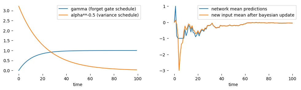
Now, let’s define a generative process of the BFN with Gaussian recursive estimation rules.
We start with an input given from a standard Gaussian parametrized using inverse variance (precision). Using precision allows to compute updates to the mean using linear combinations. Precision itself is updated by addition.
\(\mu_0, \rho_0 = 0, 1\)
The precision of likelihood \(\alpha_t\) and precision of posterior \(\rho_t\) go to infinity:
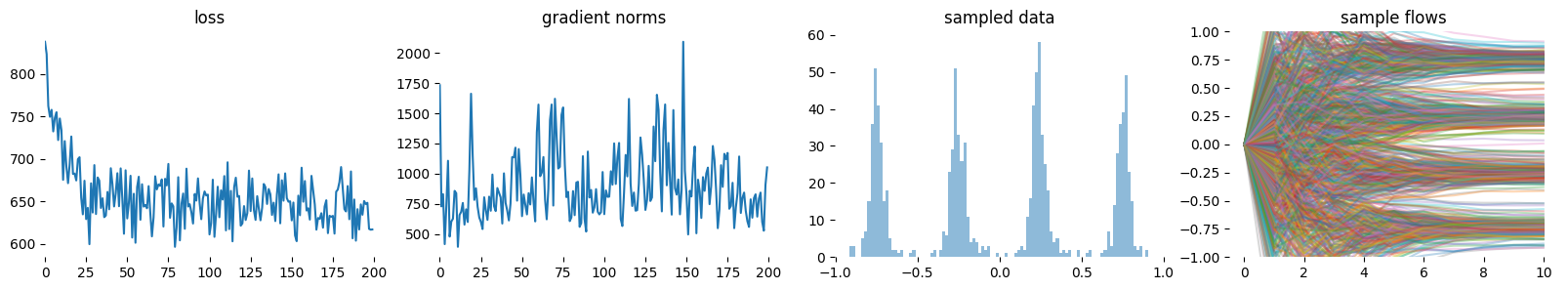
Now, let’s fit the Siren. As a distinctive feature of the BFN / diffusion, we don’t need to train on full denoising trajectories like we usually do with autoregression. We sample a datapoint, noise and a timestamp.
We minimize the divergence between the noisy version of the true data and the mean predicted by the network, with appropriate scaling.
Code
torch.manual_seed(6)torch.set_anomaly_enabled(False)flow = Siren(channels=dataset.size(1), bandwidth=10).to('cuda')dataset = dataset.to('cuda')opt = torch.optim.Adam(flow.parameters(), lr=1e-3)steps =200sigma =0.01losses = torch.zeros(steps)gnorms = torch.zeros(steps)for i inrange(steps): opt.zero_grad() minibatch = torch.arange(len(dataset)) # full batch training x = dataset[minibatch] t = torch.rand_like(x)[:, [0]]# bayesian update for input gamma =1- sigma**(2*t) std = (gamma * (1- gamma) +1e-6).sqrt() mu = gamma * x + torch.randn_like(x) * std x_ = step(flow, mu, t, gamma) scale = math.log(sigma) / sigma**(2*t) diff = x_ - x mse =-diff.square().sum(-1).sqrt() * scale loss = mse.mean() loss.backward() losses[i] = loss.item() gnorms[i] = torch.nn.utils.clip_grad_norm_(flow.parameters(), 1.0) opt.step()fig, (axl, axc, axr, axf) = plt.subplots(1, 4, figsize=(20, 3))axl.plot(losses)axl.set_title('loss')axc.plot(gnorms)axc.set_title('gradient norms')axl.set_xlim(0, steps)axc.set_xlim(0, steps)flow = flow.to('cpu')with torch.no_grad(): gen = torch.stack([generate(flow, sigma=0.01, dim=dataset.size(1), T=10, ax=axf)[-1] for _ inrange(1000)])axr.set_title('sampled data')axf.set_title('sample flows')axf.set_ylim(-1, 1)for i inrange(dataset.size(1)): axr.hist(gen[:, i].detach().numpy(), bins=100, alpha=0.5);